Scaling Timeseries Data for ISP Network Monitoring

Scaling timeseries data is a painful endeavor, and one we've had to deal with since the early days of Sonar. The short version: we collect huge volumes of network monitoring and bandwidth usage data, outgrew InfluxDB because of high series cardinality, and now run TimescaleDB on PostgreSQL with tablespaces and downsampling to keep it fast and manageable. In this post, I'll walk you through some of the failures and successes we've had, and what we're currently doing to support the growth we're seeing.

What is timeseries data?

Timeseries data is a set of data points indexed in time order. We utilize timeseries data heavily in Sonar for network monitoring and bandwidth usage monitoring, as these are both situations where you are always going to view the data ordered by time.

Generally, this type of data is stored in a special type of database that's optimized for writing and reading data structured in this way. An early platform used was RRDTool - back in the day, this was the defacto standard. It was simple to deploy, as it created files on the filesystem for every device and group of data points, and it came with built in graph generation tools.

As time went on, this became unscalable, and many new options began to crop up. Prometheus was an early option, along with Graphite and OpenTSDB, amongst many others. Many of these systems solved the same kind of needs, but in slightly different ways.

Sonar's history with timeseries data: from InfluxDB onward

In Sonar v1, we decided to use InfluxDB. This was a great option early on - it was much more performant than many of the other options available, and it was fairly easy to deploy. However, as time went on, we ran into a number of issues with InfluxDB.

First, InfluxDB uses a proprietary query language. While this is not that uncommon in timeseries databases, it is painful in many scenarios, as developers have to learn a different query language, and you have to hope that the tooling available for your programming language(s) of choice is well built, or you have to build your own.

Secondly, InfluxDB's big weakness is high series cardinality. Series cardinality is the number of different ways data can be represented - in InfluxDB, this is done using a concept of tags. For example, assume that an InfluxDB bucket has one measurement. The single measurement has two tag keys: email and status. If there are three different emails, and each email address is associated with two different statuses, the series cardinality for the measurement is 6 (3 × 2 = 6).

For our use cases, high series cardinality is very hard to escape from. We are collecting monitoring data from many devices, each with a unique ID, associated with a particular customer, each with their own unique ID, and from many different SNMP OIDs (each with their own unique OID.) When collecting data over a rapid time frame, this means the quantity of data grows extremely quickly, and the cardinality increases very rapidly. We spent a lot of time trying to optimize InfluxDB for this use case, but it was extremely challenging, and when we started on Sonar v2, we decided to look for another platform. While InfluxDB 2.0 was on the horizon, and it looked to potentially have some options to make this easier, we didn't have time to wait.

How Sonar handles timeseries data today with TimescaleDB

After a lot of evaluation and testing, we decided to use TimescaleDB. TimescaleDB was a very exciting option for us for a few reasons. One is that it's built on top of PostgreSQL, which is the underlying relational database we use for most purposes at Sonar. Secondly, all queries can be expressed as normal SQL queries, with the addition of some custom functions from TimescaleDB. This means all our existing SQL knowledge applies to TimescaleDB, and all our existing tooling is compatible with TimescaleDB. Lastly, in our testing, TimescaleDB was extremely performant, especially for our use cases in comparison to InfluxDB, and this led to the decision to move forward with this platform.

Still, even with a very performant platform, scaling timeseries data is tough. The ingestion rate for data across our entire customer base is huge - we can be bringing in millions of rows of data every minute, and without management, the data grows to an unmanageable level very quickly. Here's how we've handled it!

Scaling TimescaleDB for high-ingestion monitoring data

Storage: separating tables across SSDs with tablespaces

A place you can quickly run into issues with timeseries data is by exceeding the capabilities of the underlying hardware you're running the database on. Because so much data is being read and written so rapidly, the performance of the storage is very important.

Thankfully, because TimescaleDB is built on PostgreSQL, we were able to utilize tablespaces to separate data across multiple drives. TimescaleDB has a built in function called attach_tablespace which allows you to connect a TimescaleDB hypertable to a particular tablespace. In practice, this allowed us to separate each table we were using to a dedicated SSD, which greatly improved performance. The benefit of this approach is that we can continue to separate this out at a more granular level if needed - for example, if we had a particularly large customer that was consuming a lot of throughput, we could assign them to a dedicated disk or series of disks. We run our infrastructure in Microsoft Azure, and adding new disks on the fly is extremely simple and quick.

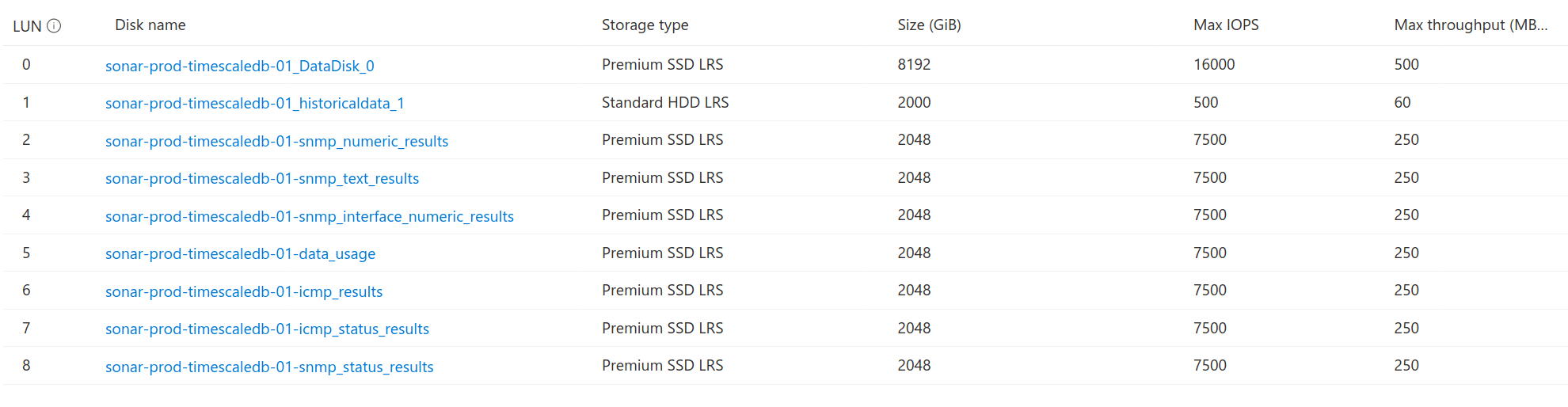
An example of the configuration for one of our TSDB servers. Each table has its own SSD, and we have a HDD connected for logs and other historical data.

Workers and actions: downsampling and compressing at scale

TimescaleDB allows you to register actions. An action is simply a PostgreSQL stored procedure that is run on a particular interval, and we use these heavily to downsample data (more on that shortly.) However, each time an action runs, it needs a background worker to be able to execute it, and if you have a lot of actions and/or databases, you can quickly exceed the available workers. You can use the timescaledb-tune tool to automatically tune your database configuration based on the hardware you're running on, but you may find you need to increase the worker count beyond the default configuration. The recommended configuration is one worker per CPU core, but depending on your CPU and the complexity of the actions you're performing, you can get away with increasing this. We skew our TimescaleDB servers towards having more cores so that we can run more workers, in comparison to our PostgreSQL servers that are more heavily skewed towards RAM.

We use actions heavily to downsample and compress data. Because we allow Sonar users to ingest data at pretty much any rate they desire, we see a lot of inbound data. This can also make queries extremely slow - even with efficient indexing, when you're trying to query data across hundreds of millions or billions of rows, the response can be very slow. It's also difficult to mentally parse this data - often, when you're looking at very recent data, very high granularity is important, but if you want to look at data from months ago, it's frequently less important. We have found that we haven't had to downsample data that heavily to improve performance and reduce storage size to a manageable level. Here's an example of a stored procedure we use to downsample data usage data.

Copy to Clipboard CREATE OR REPLACE PROCEDURE downsample_data_usage (job_id int, config jsonb)
LANGUAGE PLPGSQL
AS $$
DECLARE older interval; chunk REGCLASS; tmp_name name;
BEGIN SELECT jsonb_object_field_text (config, 'older')::interval INTO STRICT older; IF older IS NULL THEN RAISE EXCEPTION 'Config must have older'; END IF; FOR chunk IN SELECT show.oid FROM show_chunks('data_usage', older_than => older) SHOW (oid) INNER JOIN pg_class pgc ON pgc.oid = show.oid INNER JOIN pg_namespace pgns ON pgc.relnamespace = pgns.oid INNER JOIN timescaledb_information.chunks chunk ON chunk.chunk_name = pgc.relname AND chunk.chunk_schema = pgns.nspname WHERE chunk.is_compressed::bool = FALSE LOOP RAISE NOTICE 'Processing chunk: %', chunk::text; -- build name for temp table SELECT '_tmp' || relname FROM pg_class WHERE oid = chunk INTO STRICT tmp_name; -- copy downsampled chunk data into temp table EXECUTE format($sql$ CREATE UNLOGGED TABLE %I AS SELECT time_bucket('15 minutes', time) AS minutes, max(inbytes) AS inbytes, max(outbytes) AS outbytes, account_id, data_source_identifier, data_source_parent FROM %s GROUP BY minutes, account_id, data_source_identifier, data_source_parent ORDER BY minutes DESC; $sql$, tmp_name, chunk); -- clear original chunk EXECUTE format('TRUNCATE %s;', chunk); -- copy downsampled data back into chunk EXECUTE format('INSERT INTO %s(time, inbytes, outbytes, account_id, data_source_identifier, data_source_parent) SELECT * FROM %I;', chunk, tmp_name); -- drop temp table EXECUTE format('DROP TABLE %I;', tmp_name); COMMIT; RAISE NOTICE 'Reordering chunk'; PERFORM reorder_chunk(chunk, 'data_usage_account_id_time_desc_idx'); RAISE NOTICE 'Compressing chunk: %', chunk::text; PERFORM compress_chunk (chunk, true); COMMIT; END LOOP;
END
$$;

Splitting this out into manageable chunks, this procedure does the following:

Copy to Clipboard FOR chunk IN SELECT show.oid FROM show_chunks('data_usage', older_than => older) SHOW (oid) INNER JOIN pg_class pgc ON pgc.oid = show.oid INNER JOIN pg_namespace pgns ON pgc.relnamespace = pgns.oid INNER JOIN timescaledb_information.chunks chunk ON chunk.chunk_name = pgc.relname AND chunk.chunk_schema = pgns.nspname WHERE chunk.is_compressed::bool = FALSE
This iterates through each chunk in our data_usage hypertable that is older than an input value (which for us, is 1 month) and grabs each chunk that is not compressed. LOOP RAISE NOTICE 'Processing chunk: %', chunk::text; -- build name for temp table SELECT '_tmp' || relname FROM pg_class WHERE oid = chunk INTO STRICT tmp_name; -- copy downsampled chunk data into temp table EXECUTE format($sql$ CREATE UNLOGGED TABLE %I AS SELECT time_bucket('15 minutes', time) AS minutes, max(inbytes) AS inbytes, max(outbytes) AS outbytes, account_id, data_source_identifier, data_source_parent FROM %s GROUP BY minutes, account_id, data_source_identifier, data_source_parent ORDER BY minutes DESC; $sql$, tmp_name, chunk);

We now loop through each of those chunks, and create a temporary table by appending tmp to the end of the existing name. Once that's done, we use the TimescaleDB time[_](https://docs.timescale.com/latest/api#time_bucket)bucket function to group the data into 15 minute increments. Because this is counter based data, we use the max() function to grab the largest value in the window. This data is then written into the temporary table.

Copy to Clipboard -- clear original chunk EXECUTE format('TRUNCATE %s;', chunk); -- copy downsampled data back into chunk EXECUTE format('INSERT INTO %s(time, inbytes, outbytes, account_id, data_source_identifier, data_source_parent) SELECT * FROM %I;', chunk, tmp_name); -- drop temp table EXECUTE format('DROP TABLE %I;', tmp_name);

We then delete the original chunk, copy our newly downsampled data back into the old chunk, and drop the temp table.

Copy to Clipboard RAISE NOTICE 'Reordering chunk'; PERFORM reorder_chunk(chunk, 'data_usage_account_id_time_desc_idx'); RAISE NOTICE 'Compressing chunk: %', chunk::text; PERFORM compress_chunk (chunk, true);

Finally, we reorder the chunk for efficiency, before compressing it using the built in TimescaleDB compression function.

We run similar actions on the other tables we have, and the performance increase and storage size decrease is huge. For a database that had swelled to 1TB for a single customer, these actions allowed us to bring the database down to less than 200GB, and decrease query resolution time on large tables from 30 seconds to less than 3 seconds. Additional downsampling would provide additional performance boosts, but we're still evaluating the best levels to use, and trying to keep granularity as high as possible.

Frequently asked questions

Why did Sonar move from InfluxDB to TimescaleDB?

InfluxDB struggled with the high series cardinality created by monitoring many devices, customers, and SNMP OIDs, and it relied on a proprietary query language. TimescaleDB is built on PostgreSQL, supports standard SQL with a few custom functions, reuses our existing tooling, and tested as more performant for our use cases.

How does downsampling reduce storage and speed up queries?

We run TimescaleDB actions that group older chunks into 15 minute buckets, reorder, and compress them. For one customer, this brought a database from 1TB down to less than 200GB and cut query resolution on large tables from 30 seconds to under 3 seconds, while keeping recent data at high granularity.

How do you scale TimescaleDB storage for heavy ingestion?

Because TimescaleDB runs on PostgreSQL, we use tablespaces and the attach_tablespace function to place each hypertable on a dedicated SSD. Running on Microsoft Azure lets us add disks on the fly and, if needed, isolate a high-throughput customer onto their own drives.